The Basics of ETOPO.jl
ETOPO.jl builds upon the functionality of LandSea.jl to:
Download, extract and analyze the ETOPO Global Relief Model
Match it with a corresponding Land-Sea Mask
One benefit of using this package is that it pairs with GeoRegions.jl such that for small regions only the relevant region of your choosing is extracted. This saves lot of time for geographic regions of interest that are small in area relative to the globe.
Downloading automatically triggers for larger regions
For larger regions, it is often faster to download the relevant ETOPO dataset directly, rather than perform the extraction online using NCDatasets.jl (which extracts from the OPeNDAP servers). Therefore, beyond a certain threshold (currently at >10% of global area) ETOPO.jl will automatically trigger a download of the full dataset.
An Example of using ETOPO.jl
using ETOPO
using DelimitedFiles
using CairoMakie

download("https://raw.githubusercontent.com/natgeo-wong/GeoPlottingData/main/coastline_resl.txt","coast.cst")
coast = readdlm("coast.cst",comments=true)
clon  = coast[:,1]
clat  = coast[:,2]
nothing
Let us define a small GeoRegion of interest
geo = GeoRegion("AR6_SAS")The GeoRegion AR6_SAS has the following properties:
Region ID (ID) : AR6_SAS
Parent ID (pID) : GLB
Name (name) : South Asia
Bounds (N,S,E,W) : 30.0, 7.0, 100.0, 60.0
Rotation (θ) : 0.0
File Path (path) : /home/runner/.julia/packages/GeoRegions/ZNI4c/src/.files/AR6/AR6_SAS.json
Centroid (geometry.centroid) : [79.79022366522366, 21.851461038961038]
Shape (geometry.shape) : Vector{Point{2, Float64}}(13)And let us define where the ETOPO Dataset is being held
etd = ETOPODataset(path=pwd())The ETOPO Dataset {String} has the following properties:
Data Directory (path) : /home/runner/work/ETOPO.jl/ETOPO.jl/docs/build/ETOPONow, let us retrieve the ETOPO Relief data without needing to download anything
lsd = getLandSea(etd,geo)The Land-Sea Dataset (with Topography) has the following properties:
Longitude Points (lon) : Float32[60.008335, 60.025, 60.041668, 60.058334, 60.075, 60.091667, 60.108334, 60.125, 60.141666, 60.158333 … 99.84167, 99.85833, 99.875, 99.89167, 99.90833, 99.925, 99.941666, 99.958336, 99.975, 99.99167]
Latitude Points (lat) : Float32[7.008333, 7.025, 7.0416665, 7.0583334, 7.075, 7.0916667, 7.108333, 7.125, 7.141667, 7.1583333 … 29.841667, 29.858334, 29.875, 29.891666, 29.908333, 29.925, 29.941668, 29.958334, 29.975, 29.991667]
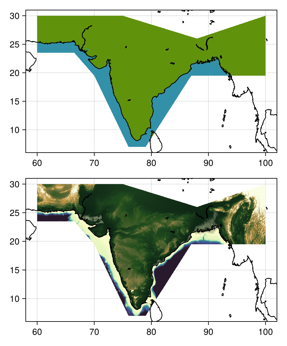
Region Size (nlon * nlat) : 2400 lon points x 1380 lat pointsAnd then now we plot both the land-sea mask (top), and the topographic height (bottom).
fig = Figure()

ax1 = Axis(
    fig[1,1],width=400,height=400*(geo.N-geo.S+2)/(geo.E-geo.W+4),
    limits=(geo.W-2,geo.E+2,geo.S-1,geo.N+1)
)
heatmap!(ax1,lsd.lon,lsd.lat,lsd.lsm,colorrange=(-0.5,1.5),colormap=:delta)
lines!(ax1,clon,clat,color=:black,linewidth=1
)

ax2 = Axis(
    fig[2,1],width=400,height=400*(geo.N-geo.S+2)/(geo.E-geo.W+4),
    limits=(geo.W-2,geo.E+2,geo.S-1,geo.N+1)
)
heatmap!(ax2,lsd.lon,lsd.lat,lsd.z ./1e3,colorrange=(-2,2),colormap=:topo)
lines!(ax2,clon,clat,color=:black,linewidth=1)

resize_to_layout!(fig)
fig