An Example of how to use RegionGrids

using GeoRegions
using RegionGrids
using DelimitedFiles
using CairoMakie

download("https://raw.githubusercontent.com/natgeo-wong/GeoPlottingData/main/coastline_resl.txt","coast.cst")
coast = readdlm("coast.cst",comments=true)
clon  = coast[:,1]
clat  = coast[:,2]
nothing

Let us define some random data:

lon = collect(0:5:360);  nlon = length(lon)
lat = collect(-90:5:90); nlat = length(lat)
data = rand(nlon,nlat)

73×37 Matrix{Float64}:
 0.0270562  0.797121   0.474738   …  0.217417   0.212276   0.471536
 0.600879   0.653407   0.166181      0.987438   0.309189   0.163279
 0.723251   0.660049   0.711799      0.384155   0.57382    0.63428
 0.462948   0.226184   0.246331      0.625997   0.509673   0.0987578
 0.576774   0.740424   0.134252      0.24509    0.775644   0.369079
 0.430942   0.682121   0.18482    …  0.786491   0.0110276  0.759566
 0.530162   0.147758   0.674606      0.140997   0.792157   0.17769
 0.648763   0.103981   0.251222      0.793199   0.125339   0.67008
 0.54477    0.401787   0.755441      0.779209   0.997329   0.415895
 0.708676   0.419967   0.428232      0.927298   0.895682   0.226484
 ⋮                                ⋱             ⋮          
 0.337432   0.284821   0.162193      0.663403   0.968179   0.969707
 0.670858   0.863976   0.937033   …  0.539578   0.0357577  0.676768
 0.505455   0.182952   0.0707261     0.0330656  0.125288   0.782244
 0.439697   0.375552   0.897063      0.387417   0.609152   0.993286
 0.557698   0.481541   0.794806      0.966444   0.390983   0.355451
 0.381448   0.884473   0.529541      0.616277   0.229714   0.456024
 0.0583404  0.765607   0.902034   …  0.930768   0.926953   0.490105
 0.38206    0.0457381  0.983659      0.404519   0.784373   0.266599
 0.444149   0.20727    0.634812      0.0284298  0.190018   0.509909

Next, we proceed to define a GeoRegion and extract its coordinates:

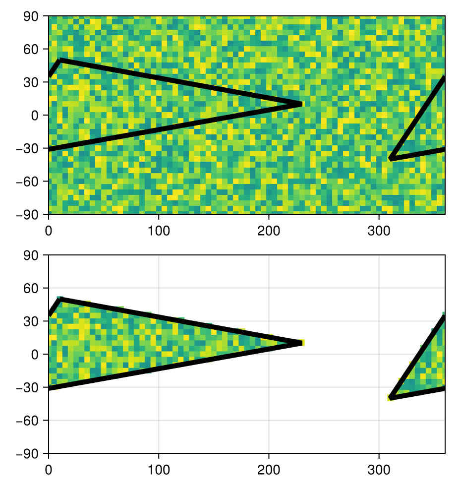
geo = GeoRegion([10,230,-50,10],[50,10,-40,50])
slon,slat = coordinates(geo) # extract the coordinates

([10.0, 230.0, -50.0, 10.0], [50.0, 10.0, -40.0, 50.0])

Following which, we can define a RegionGrid:

ggrd = RegionGrid(geo,lon,lat)

The RLinearMask Grid type has the following properties:
    Longitude Indices     (ilon) : [63, 64, 65, 66, 67, 68, 69, 70, 71, 72  …  38, 39, 40, 41, 42, 43, 44, 45, 46, 47]
    Latitude Indices      (ilat) : [11, 12, 13, 14, 15, 16, 17, 18, 19, 20, 21, 22, 23, 24, 25, 26, 27, 28, 29]
    Longitude Points       (lon) : [-50, -45, -40, -35, -30, -25, -20, -15, -10, -5  …  185, 190, 195, 200, 205, 210, 215, 220, 225, 230]
    Latitude Points        (lat) : [-40, -35, -30, -25, -20, -15, -10, -5, 0, 5, 10, 15, 20, 25, 30, 35, 40, 45, 50]
    Rotated X Coordinates    (X)
    Rotated Y Coordinates    (Y)
    Rotation (°)             (θ) : 0.0
    RegionGrid Mask       (mask)
    RegionGrid Weights (weights)
    RegionGrid Size              : 58 lon points x 19 lat points
    RegionGrid Validity		  : 465 / 1102

And then use this RegionGrid to extract data for the GeoRegion of interest:

ndata = extract(data,ggrd)

58×19 Matrix{Float64}:
   0.858423  NaN          NaN         …  NaN         NaN  NaN  NaN  NaN  NaN
 NaN           0.811148   NaN            NaN         NaN  NaN  NaN  NaN  NaN
 NaN           0.584241     0.196186     NaN         NaN  NaN  NaN  NaN  NaN
 NaN           0.738538     0.15012      NaN         NaN  NaN  NaN  NaN  NaN
 NaN           0.149309     0.10403      NaN         NaN  NaN  NaN  NaN  NaN
 NaN           0.0829975    0.241334  …  NaN         NaN  NaN  NaN  NaN  NaN
 NaN         NaN            0.314868     NaN         NaN  NaN  NaN  NaN  NaN
 NaN         NaN            0.499585     NaN         NaN  NaN  NaN  NaN  NaN
 NaN         NaN            0.326826     NaN         NaN  NaN  NaN  NaN  NaN
 NaN         NaN            0.676088       0.377023  NaN  NaN  NaN  NaN  NaN
   ⋮                                  ⋱                     ⋮            
 NaN         NaN          NaN            NaN         NaN  NaN  NaN  NaN  NaN
 NaN         NaN          NaN         …  NaN         NaN  NaN  NaN  NaN  NaN
 NaN         NaN          NaN            NaN         NaN  NaN  NaN  NaN  NaN
 NaN         NaN          NaN            NaN         NaN  NaN  NaN  NaN  NaN
 NaN         NaN          NaN            NaN         NaN  NaN  NaN  NaN  NaN
 NaN         NaN          NaN            NaN         NaN  NaN  NaN  NaN  NaN
 NaN         NaN          NaN         …  NaN         NaN  NaN  NaN  NaN  NaN
 NaN         NaN          NaN            NaN         NaN  NaN  NaN  NaN  NaN
 NaN         NaN          NaN            NaN         NaN  NaN  NaN  NaN  NaN

And we can visualize this by plotting the data

fig = Figure()

ax1 = Axis(
    fig[1,1],width=400,height=200,
    limits=(0,360,-90,90)
)
heatmap!(ax1,lon,lat,data,colorrange=(-1,1))
lines!(ax1,slon,slat,color=:black,linewidth=5)
lines!(ax1,slon.+360,slat,color=:black,linewidth=5)

ax2 = Axis(
    fig[2,1],width=400,height=200,
    limits=(0,360,-90,90)
)
heatmap!(ax2,ggrd.lon,ggrd.lat,ndata,colorrange=(-1,1))
heatmap!(ax2,ggrd.lon.+360,ggrd.lat,ndata,colorrange=(-1,1))
lines!(ax2,slon,slat,color=:black,linewidth=5)
lines!(ax2,slon.+360,slat,color=:black,linewidth=5)

resize_to_layout!(fig)
fig