The Shape of a GeoRegion
In this section, we go through process of extracting information on the shape of the GeoRegion.
Let us now setup the example
using GeoRegions
using DelimitedFiles
using CairoMakie

download("https://raw.githubusercontent.com/natgeo-wong/GeoPlottingData/main/coastline_resl.txt","coast.cst")
coast = readdlm("coast.cst",comments=true)
clon  = coast[:,1]
clat  = coast[:,2]
nothing
We load a predefined AR6 GeoRegion for Northwest North America:
geo = GeoRegion("AR6_NWN")The GeoRegion AR6_NWN has the following properties:
Region ID (ID) : AR6_NWN
Parent ID (pID) : GLB
Name (name) : Northwest North America
Bounds (N,S,E,W) : 81.0, 50.0, -105.0, -168.0
Rotation (θ) : 0.0
File Path (path) : /home/runner/work/GeoRegions.jl/GeoRegions.jl/src/.files/AR6/AR6_NWN.json
Centroid (geometry.centroid) : [-132.5882898173895, 63.942314590781585]
Shape (geometry.shape) : Vector{Point{2, Float64}}(9)Retrieving the Bounds of the GeoRegion
The bounds of the GeoRegion are given by the .N, .S, .E and .W fields in the GeoRegion struct, that denote the north and south latitude bounds, and the east and west longitude bounds.
geo.N,
geo.S,
geo.E,
geo.W
(81.0, 50.0, -105.0, -168.0)Retrieving the Rotation
By default, there is no rotation projection passed onto the GeoRegion. However, if you have passed on a rotation projection, you can retrieve it via the field .θ, which is given in degrees.
geo.θ0.0Retrieving the Centroid
We can also retrieve the longitude/latitude coordinates of the centroid of the GeoRegion using the .geometry.centroid field.
lonc,latc = geo.geometry.centroid2-element Point{2, Float64} with indices SOneTo(2):
-132.5882898173895
63.942314590781585Retrieving the coordinates of a GeoRegion
Using the function coordinates(), we are able to retrieve the coordinates of the vertices that define the shape of the GeoRegion. In the below example, we plot the longitude and latitude points.
lon,lat = coordinates(geo)

aspect = (geo.E-geo.W+4)/(geo.N-geo.S+4)
fig = Figure()
ax = Axis(
    fig[1,1],width=750,height=750/aspect,
    limits=(geo.W-2,geo.E+2,geo.S-2,geo.N+2),
    xlabel = "Longitude / º", ylabel = "Latitude / º"
)
lines!(ax,clon,clat,color=:black,linewidth=3)
lines!(ax,lon,lat,linewidth=5)
scatter!(ax,lonc,latc,markersize=20)
resize_to_layout!(fig)
fig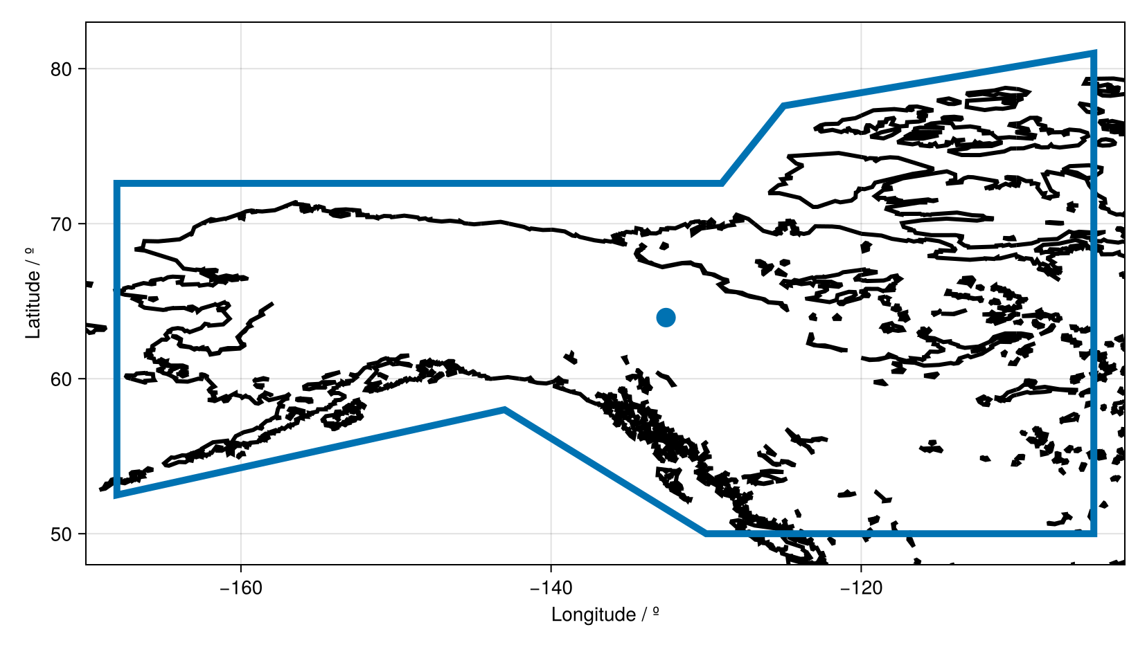
This plotting works on maps where the projection is equirectangular. However, there are many different map projections, and so we can specify the number of segments n on each side of the shape using the keyword argument n in order to ensure during plotting that is plotted correctly on the projection.
nlon,nlat = coordinates(geo,n=50)
length(lon), length(nlon)
(9, 401)Number of Points
The shape is defined by 8 sides. Therefore there are by default 8 + 1 = 9 coordinate points to close the polygon. If we specify 50 segments a side, we therefore have 400 + 1 = 401 coordinate points to close the polygon.
See the API here