Rectilinear Grids for Data Extraction

The most straightforward of the RegionGrid types is the RectilinearGrid. This is the type that is used for most datasets on a rectilinear longitude/latitude grid. Examples of such datasets include:

Level 3 products from the Global Precipitation Measurement Mission
Final regridded products from reanalysis such as ERA5 and MERRA2
Model output from simple climate models such as Isca and SpeedyWeather.jl

Basically, for each of these datasets, the data is given in such a way that the coordinates of the grid can be expressed via two vectors/ranges:

A vector/range of longitudes
A vector/range of latitudes

julia

using GeoRegions
using RegionGrids
using CairoMakie

Creating Rectilinear Grids

A Rectilinear Grid can be created as follows:

ggrd = RegionGrid(geo,lon,lat)

where geo is a GeoRegion of interest that is found within the domain defined by the longitude and latitude grid vectors.

julia

lon = collect(0:5:359);  nlon = length(lon)
lat = collect(-90:5:90); nlat = length(lat)
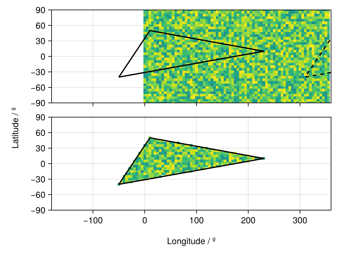
geo = GeoRegion([10,230,-50,10],[50,10,-40,50])

ggrd = RegionGrid(geo,lon,lat)

The RLinearMask Grid type has the following properties:
    Longitude Indices     (ilon) : [63, 64, 65, 66, 67, 68, 69, 70, 71, 72  …  38, 39, 40, 41, 42, 43, 44, 45, 46, 47]
    Latitude Indices      (ilat) : [11, 12, 13, 14, 15, 16, 17, 18, 19, 20, 21, 22, 23, 24, 25, 26, 27, 28, 29]
    Longitude Points       (lon) : [-50, -45, -40, -35, -30, -25, -20, -15, -10, -5  …  185, 190, 195, 200, 205, 210, 215, 220, 225, 230]
    Latitude Points        (lat) : [-40, -35, -30, -25, -20, -15, -10, -5, 0, 5, 10, 15, 20, 25, 30, 35, 40, 45, 50]
    Rotated X Coordinates    (X)
    Rotated Y Coordinates    (Y)
    Rotation (°)             (θ) : 0.0
    RegionGrid Mask       (mask)
    RegionGrid Weights (weights)
    RegionGrid Size              : 57 lon points x 19 lat points
    RegionGrid Validity		  : 451 / 1083

The API for creating a Rectilinear Grid can be found here

What is in a Rectilinear Grid?

RegionGrids.RectilinearGrid Type

julia

RectilinearGrid <: RegionGrid

A RectilinearGrid is a RegionGrid that is created based on rectilinear longitude/latitude grids. It has its own subtypes: RectGrid, TiltGrid and PolyGrid.

All RectilinearGrid types contain the following fields:

lon - A Vector of Floats, defining the longitude vector describing the region.
lat - A Vector of Floats, defining the latitude vector describing the region.
ilon - A Vector of Ints, defining the indices used to extract the longitude vector from the input longitude vector.
ilat - A Vector of Ints, defining the indices used to extract the latitude vector from the input latitude vector.
mask - An Array of NaNs and 1s, defining the gridpoints in the RegionGrid where the data is valid.
weights - A Vector of Floats, defining the latitude-weights of each valid point in the grid. Will be NaN if outside the bounds of the GeoRegion used to define this RectilinearGrid.
X - A Vector of Floats, defining the X-coordinates (in meters) of each point in the "derotated" RegionGrid about the centroid for the shape of the GeoRegion.
Y - A Vector of Floats, defining the Y-coordinates (in meters) of each point in the "derotated" RegionGrid about the centroid for the shape of the GeoRegion.
θ - A Float storing the information on the angle (in degrees) about which the data was rotated in the anti-clockwise direction. Mathematically, it is rotation - geo.θ.

source

We see that in a RectilinearGrid type, we have the lon and lat fields that defined the longitude and latitude vectors that have been cropped to fit the GeoRegion bounds.

julia

ggrd.lon, ggrd.lat

([-50, -45, -40, -35, -30, -25, -20, -15, -10, -5  …  185, 190, 195, 200, 205, 210, 215, 220, 225, 230], [-40, -35, -30, -25, -20, -15, -10, -5, 0, 5, 10, 15, 20, 25, 30, 35, 40, 45, 50])

An example of using Rectilinear Grids

Say we have some sample data, here randomly generated.

julia

data = rand(nlon,nlat)

72×37 Matrix{Float64}:
 0.290019  0.531737   0.863422  0.875342   …  0.387476   0.579014  0.957663
 0.892206  0.780838   0.710163  0.349509      0.766642   0.881841  0.428139
 0.532511  0.9543     0.256315  0.547556      0.500861   0.12039   0.880504
 0.238221  0.340806   0.395366  0.844729      0.537302   0.570758  0.768156
 0.972486  0.741446   0.764157  0.656752      0.473778   0.952143  0.500683
 0.675901  0.0446133  0.700759  0.34068    …  0.915844   0.2856    0.183354
 0.141882  0.659196   0.830121  0.427681      0.0519131  0.955004  0.29897
 0.62238   0.788223   0.856918  0.985316      0.810153   0.337734  0.150978
 0.864406  0.321432   0.487837  0.760536      0.309275   0.20043   0.589917
 0.682755  0.341155   0.948315  0.926153      0.40366    0.981268  0.125615
 ⋮                                         ⋱             ⋮         
 0.782883  0.769686   0.213261  0.0308808     0.761774   0.432126  0.877195
 0.998696  0.255472   0.43763   0.34865       0.742388   0.876634  0.375893
 0.710652  0.716492   0.955429  0.449564   …  0.396214   0.260832  0.769747
 0.853264  0.509834   0.245726  0.963825      0.748513   0.20723   0.189513
 0.924109  0.194019   0.212178  0.102164      0.312784   0.320979  0.363403
 0.344816  0.916852   0.334233  0.666425      0.207642   0.56607   0.592557
 0.403109  0.871866   0.207246  0.456931      0.726259   0.982984  0.995632
 0.354437  0.167404   0.636111  0.506391   …  0.346254   0.930364  0.796509
 0.226417  0.0365091  0.242117  0.202493      0.9284     0.980195  0.641897

We extract the valid data within the GeoRegion of interest that we defined above:

julia

ndata = extract(data,ggrd)

57×19 Matrix{Float64}:
   0.131637  NaN          NaN          …  NaN         NaN  NaN  NaN  NaN  NaN
 NaN           0.477372   NaN             NaN         NaN  NaN  NaN  NaN  NaN
 NaN           0.869184     0.0995539     NaN         NaN  NaN  NaN  NaN  NaN
 NaN           0.15509      0.969218      NaN         NaN  NaN  NaN  NaN  NaN
 NaN           0.0789877    0.60641       NaN         NaN  NaN  NaN  NaN  NaN
 NaN           0.626356     0.857419   …  NaN         NaN  NaN  NaN  NaN  NaN
 NaN         NaN            0.36496       NaN         NaN  NaN  NaN  NaN  NaN
 NaN         NaN            0.299786      NaN         NaN  NaN  NaN  NaN  NaN
 NaN         NaN            0.671398      NaN         NaN  NaN  NaN  NaN  NaN
 NaN         NaN            0.463152        0.614852  NaN  NaN  NaN  NaN  NaN
   ⋮                                   ⋱                     ⋮            
 NaN         NaN          NaN             NaN         NaN  NaN  NaN  NaN  NaN
 NaN         NaN          NaN             NaN         NaN  NaN  NaN  NaN  NaN
 NaN         NaN          NaN          …  NaN         NaN  NaN  NaN  NaN  NaN
 NaN         NaN          NaN             NaN         NaN  NaN  NaN  NaN  NaN
 NaN         NaN          NaN             NaN         NaN  NaN  NaN  NaN  NaN
 NaN         NaN          NaN             NaN         NaN  NaN  NaN  NaN  NaN
 NaN         NaN          NaN             NaN         NaN  NaN  NaN  NaN  NaN
 NaN         NaN          NaN          …  NaN         NaN  NaN  NaN  NaN  NaN
 NaN         NaN          NaN             NaN         NaN  NaN  NaN  NaN  NaN

And now let us visualize the results.

julia

slon,slat = coordinates(geo) # extract the coordinates
fig = Figure()

ax1 = Axis(
    fig[1,1],width=450,height=150,
    limits=(-180,360,-90,90)
)
heatmap!(ax1,lon,lat,data,colorrange=(-1,1))
lines!(ax1,slon,slat,color=:black,linewidth=2)
lines!(ax1,slon.+360,slat,color=:black,linewidth=2,linestyle=:dash)

hidexdecorations!(ax1,ticks=false,grid=false)

ax2 = Axis(
    fig[2,1],width=450,height=150,
    limits=(-180,360,-90,90)
)
heatmap!(ax2,ggrd.lon,ggrd.lat,ndata,colorrange=(-1,1))
lines!(ax2,slon,slat,color=:black,linewidth=2)

Label(fig[3,:],"Longitude / º")
Label(fig[:,0],"Latitude / º",rotation=pi/2)

resize_to_layout!(fig)
fig

Rectilinear Grids for Data Extraction ​

Creating Rectilinear Grids ​

What is in a Rectilinear Grid? ​

An example of using Rectilinear Grids ​

Rectilinear Grids for Data Extraction

Creating Rectilinear Grids

What is in a Rectilinear Grid?

An example of using Rectilinear Grids