Unstructured Grids for Data Extraction
There are also RegionGrid types without an actual grid, maybe there are a set of coordinates and geometries that define the corners or the centres of a mesh, such as:
- Model output from climate models such as cubed-sphere mesh output of the Community Earth Systems Model 2 (CESM2).
Basically, for each of these datasets, the data is given in such a way that the coordinates of the grid can be expressed via:
- A Vector of
Point2types, with eachPoint2type containing (lon,lat)
using GeoRegions
using RegionGrids
using CairoMakie
Creating Unstructured Grids
A Unstructured Grid can be created as follows:
ggrd = RegionGrid(geo,Point2.(lon,lat))where geo is a GeoRegion of interest that is found within the domain defined by the longitude and latitude grid vectors.
lon = collect(10:20:360); nlon = length(lon)
lat = collect(-80:20:90); nlat = length(lat)

glon = zeros(nlon,nlat); glon .= lon;  glon = glon[:]
glat = zeros(nlon,nlat); glat .= lat'; glat = glat[:]

plon = glon .+ 14rand(nlon*nlat) .- 7
plat = glat .+ 14rand(nlon*nlat) .- 7

geo = GeoRegion([10,100,-80,10],[50,10,-40,50])

iggrd = RegionGrid(geo,Point2.(glon,glat))
pggrd = RegionGrid(geo,Point2.(plon,plat))
The VectorMask Grid type has the following properties:
Indices (ipoint) : [70, 71, 73, 74, 89, 90, 91, 92, 93, 94, 108, 109]
Longitude Points (lon) : [-45.34307655667226, -36.77876709238751, 16.300715051773935, 27.140990278062965, -31.101564896462378, -11.900811333392994, 16.170649910309834, 23.643136174094188, 53.817125009318445, 74.87879312706845, -4.533605078450307, 10.384761114582073]
Latitude Points (lat) : [-20.418087077696008, -15.88712532473336, 3.6409350931376494, 2.0581211352587996, -0.07520706019646362, 6.0719428622373925, 16.296267073610878, 26.01989307767802, 13.234261758522521, 17.64158636983985, 24.527264283725454, 34.76597950091516]
Rotated X Coordinates (X)
Rotated Y Coordinates (Y)
Rotation (°) (θ) : 0.0
RegionGrid Weights (weights)
RegionGrid Size : (12,) pointsThe API for creating a Unstructured Grid can be found here
What is in a Unstructured Grid?
RegionGrids.UnstructuredGrid Type
UnstructuredGrid <: RegionGridA UnstructuredGrid is a RegionGrid that is created based on an unstructured grid often used in cubed-sphere or unstructured-mesh grids.
All UnstructuredGrid type will contain the following fields:
lon- A Vector ofFloats, defining the longitudes for each point in the RegionGrid that describe the region.lat- A Vector ofFloats, defining the latitude for each point in the RegionGrid that describe the region.ipoint- A Vector ofInts, defining the indices of the valid points from the original unstructured grid that were extracted into the RegionGrid.weights- A Vector ofFloats, defining the latitude-weights of each valid point in the grid. Will be NaN if outside the bounds of the GeoRegion used to define this RectilinearGrid.X- A Vector ofFloats, defining the X-coordinates (in meters) of each point in the "derotated" RegionGrid about the centroid for the shape of the GeoRegion.Y- A Vector ofFloats, defining the Y-coordinates (in meters) of each point in the "derotated" RegionGrid about the centroid for the shape of the GeoRegion.θ- AFloatstoring the information on the angle (in degrees) about which the data was rotated in the anti-clockwise direction. Mathematically, it isrotation - geo.θ.
We see that in a UnstructuredGrid type, we have the lon and lat vectors that defined the longitude and latitude points that are within the GeoRegion.
ggrd.longgrd.latAn example of using Unstructured Grids
Say we have some sample data, here randomly generated.
data = rand(nlon,nlat)[:]162-element Vector{Float64}:
0.21312057522925842
0.6800326962507157
0.43407134407142245
0.025933254333968536
0.676470701150551
0.4578902879765151
0.9621453905370656
0.3249231790620096
0.3163746337516481
0.2549750700831279
⋮
0.8317888337429427
0.6320400593375758
0.22120888589882992
0.1669278443669009
0.8794258933745993
0.48408382743659684
0.01509470529196466
0.3189816977880584
0.13296466355021386We extract the valid data within the GeoRegion of interest that we defined above:
ndata = extract(data,iggrd)
pdata = extract(data,pggrd)
12-element Vector{Float64}:
0.6835266403893645
0.19962648634209257
0.7515520344336604
0.5378624142662117
0.838261297872362
0.1482140109754707
0.6406531374951079
0.9753354387320468
0.7218324287917494
0.4392853911888741
0.0770502206696152
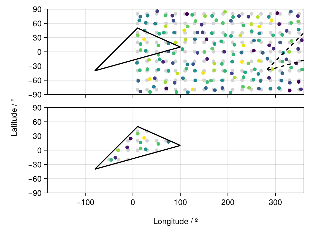
0.7750688546815884And now let us visualize the results.
slon,slat = coordinates(geo) # extract the coordinates
fig = Figure()

ax1 = Axis(
    fig[1,1],width=450,height=150,
    limits=(-180,360,-90,90)
)
scatter!(ax1,glon,glat,color=:lightgrey)
scatter!(ax1,plon,plat,color=data)
lines!(ax1,slon,slat,color=:black,linewidth=2)
lines!(ax1,slon.+360,slat,color=:black,linewidth=2,linestyle=:dash)

hidexdecorations!(ax1,ticks=false,grid=false)

ax2 = Axis(
    fig[2,1],width=450,height=150,
    limits=(-180,360,-90,90)
)
scatter!(ax2,iggrd.lon,iggrd.lat,color=:lightgrey)
scatter!(ax2,pggrd.lon,pggrd.lat,color=pdata)
lines!(ax2,slon,slat,color=:black,linewidth=2)

Label(fig[3,:],"Longitude / º")
Label(fig[:,0],"Latitude / º",rotation=pi/2)

resize_to_layout!(fig)
fig